
Which Phone Numbers Are More Likely to Answer Your Call?
Generating Contactability Scores Using Machine Learning
by Shigeki Kamata, Data Scientist
August 5, 2020
Introduction
If you need to make a phone call for your business, what are the chances the person will pick up your call? There are many business situations where this problem will come into play. Say you have a list of phone numbers that you want to call to raise money for charity. You want to talk to as many people from the list as possible with limited time and a limited number of staff to make the phone calls. Perhaps, for example, your list contains 700,000 phone numbers and you only have a week and five staff members to make your phone calls. A good plan would be to begin by calling the people who are most likely to answer your call rather than starting from the top of the list. A Contactability Score, as described in this paper, makes this possible by evaluating what we know about a given phone number and deriving a score. "Contactability Scores" are indicators of how likely a given phone number is to be answered. By sorting your list according to the contactability scores, you will be more likely to start your phone call campaign with successful calls.
A contactability score (CS) is a score that indicates how likely a person is to answer a phone call from an unknown caller. We can provide a CS for any phone number by utilizing machine learning algorithms. In this article, we are going to explore how contactability scores are generated by taking a closer look at the machine learning process.
In the field of data science, this kind of task is called Unsupervised Machine Learning. We train a machine learning algorithm by feeding it phone log data that shows whether people have answered (or not answered) phone calls in the past. In a way, this is like a teacher giving a student a problem set and its solution. The machine learning algorithm "learns" from this historical data and builds an algorithm to predict whether or not a person at a given number will answer a phone call. Let's begin by exploring the process of machine learning. The following is a simplified explanation of one technique that can be used to produce contactability scores. While PacificEast uses machine learning in its score development process, what follows is not necessarily an exact match of how PacificEast Research generates their contactability scores as the exact formula and nature of our Contactability Score is proprietary.
This article is intented for those who are interested in and new to machine learning. I will go over basic steps of machine learning model making. First, I will discuss how to prepare and observe the data set. Secondly, I will create five different machine learning models that are commonly used in data science. I will also briefly explain the basic intuition about how each machine learning model is formulated. Finally, I will use those models to predict the contactability scores for given phone numbers and see how accurate the predictions are.
Data Preparation
Throughout this article we will use Python as the platform. You will see Python codes in blue boxes. Those are the actual codes that handle the data and generate machine learning models. For each coding section, I will give a concise explanation about what the code section is doing so that you don't have to understand the meaning of the code line by line.
First, let's start by loading the necessary packages and data sets for this
analysis:
# Import the librariesimport numpy as np
import matplotlib.pyplot as plt
import pandas as pd
import warnings
warnings.filterwarnings('ignore')
# Load the datasetraw_df = pd.read_csv('raw_data.csv')
raw_df in the code block above
contains the data of about 40,000 phone numbers and whether or not the owners
of the phone numbers answered the phone call in the past. Let's take some
samples from the dataset and see what the data looks like (for privacy reasons,
the last four digits of the phone numbers are masked):
print_df = raw_df.sample(5, random_state=1)
print_df['PHONE'] = (print_df['PHONE']).astype(str).str[0:3] + ' - ' + (print_df['PHONE']).astype(str).str[3:6] + " - ****"
print_df
|
PHONE |
ANSWER |
|
|
4773 |
760 - 975 - **** |
0 |
|
38007 |
818 - 848 - **** |
0 |
|
7819 |
949 - 599 - **** |
1 |
|
5666 |
720 - 331 - **** |
1 |
|
29945 |
650 - 380 - **** |
0 |
We want the machine learning algorithm to learn from this data set and make predictions on unknown numbers in the future. However, it is unlikely for a machine learning algorithm to grasp patterns based on phone numbers alone. So, we will add some columns to the data by deriving some more information from the phone number.
# Import the derived datasetdf = pd.read_csv('derived_data.csv')
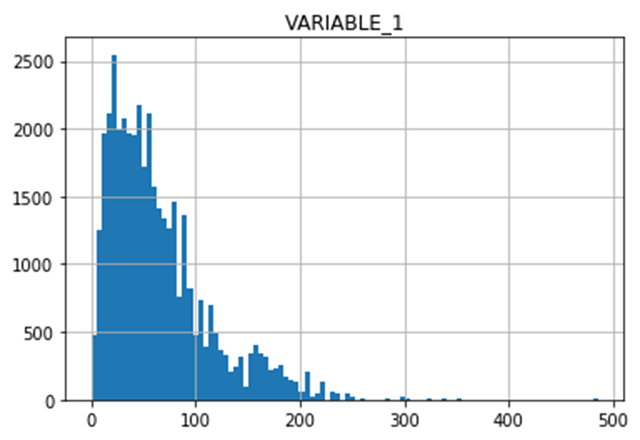
The derived dataset looks like this. The first two of the four new columns are numerical data while the last two are categorical data.
print_df = df.sample(5,random_state=1)
print_df['PHONE'] = (print_df['PHONE']).astype(str).str[0:3] + ' - ' + (print_df['PHONE']).astype(str).str[3:6] + " - ****"
print_df
|
PHONE |
VARIABLE_1 |
VARIABLE_2 |
VARIABLE_3 |
|
VARIABLE_4 |
ANSWER |
|
|
34773 |
760 - 975 - **** |
49.3966 |
29.7727 |
C |
|
3 |
0 |
|
38007 |
818 - 848 - **** |
58.6207 |
32.6190 |
B |
|
1 |
0 |
|
7819 |
949 - 599 - **** |
64.4537 |
41.0393 |
A |
|
4 |
1 |
|
5666 |
720 - 331 - **** |
15.1930 |
44.1824 |
A |
|
0 |
1 |
|
29945 |
650 - 380 - **** |
159.7520 |
20.3375 |
A |
|
0 |
0 |
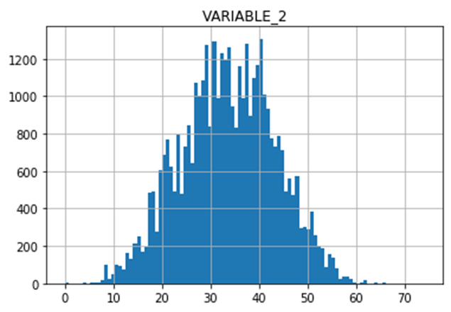
Let's take a look at the distributions of the new variables:
plt.hist(df.VARIABLE_1, bins = 100)
plt.title("VARIABLE_1")
plt.grid(True)
plt.show()
plt.hist(df.VARIABLE_2, bins = 100)
plt.title("VARIABLE_2")
plt.grid(True)
plt.show()
df.VARIABLE_3.value_counts()
A 23468B 8777C 7761Name: VARIABLE_3, dtype: int64df.VARIABLE_4.value_counts()
1 113293 110190 108504 45252 2283Name: VARIABLE_4, dtype: int64
In order for a machine learning algorithm to learn and generate a predictive algorithm (in data science, we call it "training" the model), we need to process the data so that it is digestible for the machine.
# Define numerical and categorical columnsnum_cols = ['VARIABLE_1', 'VARIABLE_2']
cat_cols =['VARIABLE_3', 'VARIABLE_4']
# Define X and yX = df[num_cols + cat_cols]
y = df.ANSWER
from sklearn.pipeline import Pipeline
from sklearn.impute import SimpleImputer
from sklearn.preprocessing import StandardScaler, OneHotEncoder
from sklearn.compose import ColumnTransformer
numeric_transformer = Pipeline(steps=[
('imputer', SimpleImputer(strategy='median')),
('scaler', StandardScaler())])
categorical_transformer = Pipeline(steps=[
('imputer', SimpleImputer(strategy='constant', fill_value='missing')),
('onehot', OneHotEncoder(handle_unknown='ignore'))])
preprocessor = ColumnTransformer(
transformers=[
('num', numeric_transformer, num_cols),
('cat', categorical_transformer, cat_cols)])
Train Machine Learning Models
In this section, we will build and train several predictive models utilizing machine learning algorithms and see how well they predict the result. In order to do so, we separate our dataset into two parts; training set and test set. We use the training set to formulate the predictive algorithm. Then we use the test set to make predictions and check if the predictions are correct. For this article, let's take 80% of the data for training and the rest for testing. For each potential model building method we will highlight some of the advantages and disadvantages a given modelling method has over the others.
# Separate data into training and validation setsfrom sklearn.model_selection import train_test_split
X_train, X_test, y_train, y_test = train_test_split(X,y, test_size=0.2,
random_state=0, stratify=y)
Logistic Regression
Model Methodology
Logistic Regression is a statistic model to classify data into two categories. We compute the impact each variable has on the result. The resulting value is expressed in the form of a linear combination of the variables. Then we transform this equation using a function called the logit function so that the resulting value fits in the 0-1 range.
Advantage:
Easy to interpret the model
Disadvantages:
Hard to capture complex relationships
Works poorly with correlated data
from sklearn.linear_model import LogisticRegression
logistic = LogisticRegression(random_state = 0)
Random Forest
Model Methodology
Random Forest is a type of ensemble learning where we utilize many decision trees and draw a conclusion based on how each decision tree "votes". A decision tree is like an upside-down tree shaped flow-chart whose nodes have questions like "Is the VARIABLE_1 greater than 13.5?" or "Is VARIABLE_3 B?". By answering the questions and descending to the bottom of the tree, you get to the conclusion such as "ANSWER = 1" or "ANSWER = 0".
We start by creating N decision tree algorithms, which get trained with M random elements from the training set. Each trained decision tree makes a prediction and our final prediction is chosen according to the majority vote of the N trees. Each individual decision tree's prediction ability is usually not very good since its data input is limited to a subset of the entire dataset. However, if we let the trees vote for the conclusion, the majority vote comes to a fairly accurate prediction.
Advantages:
High performance and accuracy in general
Can automatically handle missing values
Less data preprocessing needed
Disadvantages:
Difficult to interpret, black box approach
Can overfit the training data
from sklearn.ensemble import RandomForestClassifier
rf = RandomForestClassifier(bootstrap=False, ccp_alpha=0.0, class_weight=None,criterion='gini', max_depth=10, max_features='auto', max_leaf_nodes=None, max_samples=None, min_impurity_decrease=0.0, min_impurity_split=None, min_samples_leaf=2, min_samples_split=2, min_weight_fraction_leaf=0.0, n_estimators=100, n_jobs=None, oob_score=False, random_state=None, verbose=0, warm_start=False)
XGBoost
Model Methodology
Just like Random Forest, XGBoost is a decision-tree-based ensemble Machine Learning algorithm. XGboost produces a predictive model in the form of an ensemble of weak predictors. It builds the model by revising its parameters iteratively in many stages where the algorithm studies the differences between the prediction and the answer and resets the parameter so that it minimizes the difference.
Advantages:
It tends to perform very well
It can handle missing data well
Disadvantages:
It is generally hard to interpret
It has many hyperparameters and is hard to tune properly
from xgboost import XGBClassifier
xgb = XGBClassifier(n_estimators=500, learning_rate=0.05, n_jobs = -1)
K Nearest Neighbor
Model Methodology
The K Nearest Neighbor (KNN) algorithm calculates the distance
between a new data point and all the elements of the training set. The distance
can be measured with several different metrics, such as Euclidean, Manhattan,
etc. According to the chosen metric, the algorithm selects the k nearest
elements, where k can be specified by the user. The k elements then vote for
the class to which the new data point should belong. In short, KNN carries out
classification by this element should be 1 (or 0) because 90% of its neighbors
are 1 (or 0) .
Advantages:
Fast. No prior training needed
Disadvantages:
Does not work well with higher dimensions or large data sets, as
it gets harder to calculate the distances
from sklearn.neighbors import KNeighborsClassifier
knn = KNeighborsClassifier(algorithm='auto', leaf_size=30, metric='minkowski',
metric_params=None, n_jobs=None, n_neighbors=22, p=2, weights='uniform')
Artificial Neural Network
Artificial Neural Network is an algorithm that is inspired by biological nervous systems, such as the human brain. The basic unit of computation is the neuron. It receives input from some other neuron (or from an external source) and computes an output. Each input has an associated weight (w), which is assigned on the basis of its relative importance to other inputs. The node applies a function f to the weighted sum of its inputs.
Advantage:
It performs very well for audio, text, and image data
Disadvantages:
As with regression, neural networks require very large amounts of
data to train, so it's not treated as a general-purpose algorithm
# MLP classifierfrom sklearn.neural_network import MLPClassifier
mlp = MLPClassifier(hidden_layer_sizes=(20,20),max_iter=500)
Evaluation of five Machine Learning Algorithms
With all the algorithms ready, we will now make predictions about whether or not the person will answer a phone call. Since our primary goal is to sort the phone number list from most to least likely to answer a phone call we will introduce a scoring criteria that suits our objective. First, we define the Percentile Answer Ratio graph (PAR graph). The PAR graph shows the percent of "good" phone numbers that are included when you limit the phone number list to the top x% by the CS. If you call 30% of the phone numbers on the list without any proper sorting, it is expected that 30% of all the good numbers will be included in your subset. If our machine learning algorithm successfully sorts the list, then the ratio of the good numbers in your subset will be more than 30%. The PAR graph is an indication of how much improvement we can obtain by sorting the phone numbers according to the CSs the model indicates. Let's take a look at the evaluation process step-by-step:
Making Predictions
We will take the case of
the Logistic Regression model as an example. First, we train the model by
feeding it with the training set. The training set provide "problems"
and "answers" to the model.X_train corresponds to the problems
and y_train corresponds to the answers. By looking
at the problem and the answers, the model uses its unique model-forming
algorithm and forms a predictor that predicts the value of ANSWER column of
unknown input. After that, we let the model predict the result using the test
set (X_test) and see
how well or poorly the model predicts the ANSWER column.
my_model = Pipeline(steps=[('preprocessor', preprocessor),
('classifier', logistic)])
my_model.fit(X_train, y_train)
predictions = my_model.predict_proba(X_test)[:,1]
In the
second line of the code section above, the model learned from X_train and y_train and
formed the predictive model. In the last line, we feed X_test to
the model and let it predict the values of the ANSWER column. Note that we
don't give the model y_test, which contain the
correct values of the ANSWER column. Finally, prediction vector was created by the
model. This vector contains the predicted values of the phone numbers in X_test. The
prediction is given in the form of probability, as shown below. The number
0.19451494 means that the model predicts there is a 19.4% chance the owner of
the first phone number in the list will answer the unknown call.
predictions
array([0.19451494, 0.16487552, 0.1971855 , ..., 0.17340611, 0.41838922, 0.46196348])Distribution
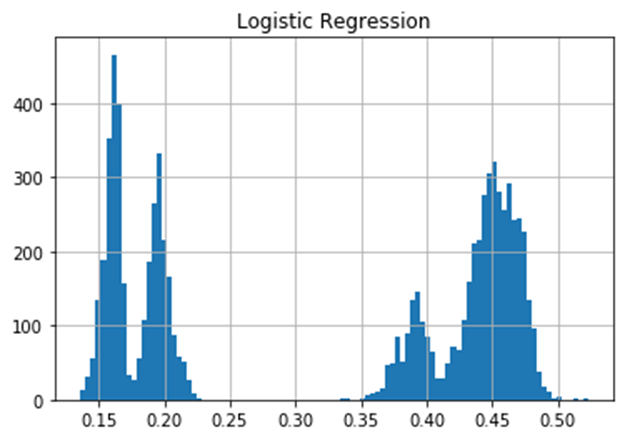
Having made the prediction, we will take a look at the distribution of the scores.
plt.hist(predictions, bins = 100)
plt.title("Distribution of Contactability Score")
plt.grid(True)
plt.show()
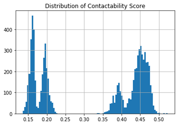
The histogram above shows the distribution of the CS. It indicates there are two (or possibly four) distinctive trends; one around 0.17 and the other around 0.45. However, since our interest is not so much on binary prediction (whether someone answers the call or not) but rather on sorting the phone numbers according to the contactability score, we will not explore the shape of the distribution further. Instead, we need to find out how much improvement we can get if we sort the phone numbers by this score.
PAR Graph
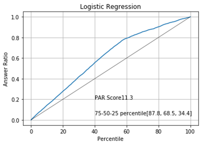
We need some measurement to assess how well the model sorts the phone numbers. For this purpose, we will define a graph called the Percentile Answer Ratio graph (PAR graph). A PAR graph evaluates a sorting by calculating how much improvement you get with the sorting compared to non-sorted phone list. More specifically, the PAR graph returns the percentage of "good" phone numbers out of all the good phone numbers in the entire list for a given percentage by which we limit the phone number list. Let's take a look at the PAR graph of the Logistic Regression model:
def par_graph(y, y_pred, model_name):
data = {'y':y, 'y_pred':y_pred}
df = pd.DataFrame(data)
sorted_df =df.sort_values(by = 'y_pred', axis=0, ascending=False)
total_answered = sum(sorted_df.y == 1)
ratios = []
for i in range(0,101):
percentile = round(sorted_df.shape[0] * (i/100) )
new_ratio = sum(sorted_df.y[0:percentile] == 1) / total_answered
ratios.append(new_ratio)
par_data = pd.DataFrame()
par_data['Percentile'] = range(0,101)
par_data['Ratio'] = ratios
par_score = sum(par_data['Ratio']) - 50
key_ratios = [round(ratios[i]* 100 ,1) for i in [75, 50, 25]]
plt.plot(par_data['Percentile'], par_data['Ratio'])
plt.xlabel('Percentile')
plt.ylabel('Answer Ratio')
plt.title(model_name)
plt.text(40, .2, "PAR Score" + str(round(par_score, 1)))
plt.text(40, .05, "75-50-25 percentile" + str(key_ratios))
plt.plot([0,100],[0,1], color='black',linewidth= 0.5)
plt.grid(True)
plt.show()
# Show PAR graphpar_graph(y_test, predictions, "Percentile Answer Ratio Graph")
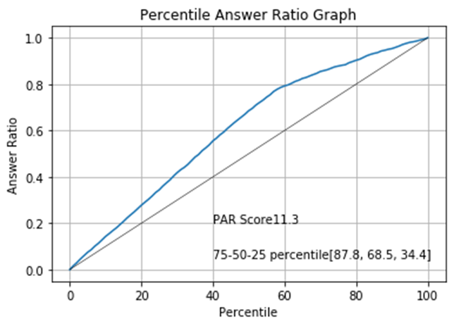
The black straight line indicates the expected outcome of the calling campaign if we make phone calls randomly. For example, limiting the call to 40% is expected to reduce the number of successful calls to also 40%. The blue curve indicates the expected outcome if we sort the list according to the contactability score given by our logistic regression. It shows that if we limit the number of calls to 40%, nearly 60% of the successful calls are preserved in the subset. The "75-50-25 percentile" show what percent of good phone numbers are retained in the subset when we limit the phone number list to the 75, 50 or 25%. The PAR score corresponds to the area between the black line and the blue curve. Generally, a higher PAR score means better sorting.
Model-wise Comparison
For the other models, we will take the same steps as we did on the Logistic Regression.
models = [(logistic, 'Logistic Regression'),
(rf, 'Random Forest'),
(xgb, 'XGBoost'),
(knn, 'K Nearest Neighbor'),
(mlp, 'Neural network')]
for model in models:
my_model = Pipeline(steps=[('preprocessor', preprocessor),
('classifier', model[0])])
my_model.fit(X_train, y_train)
predictions = my_model.predict_proba(X_test)[:,1]
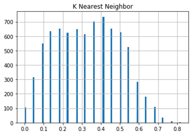
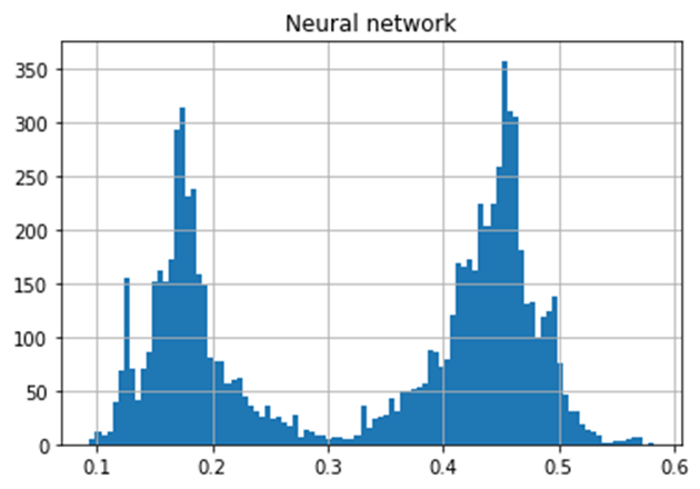
plt.hist(predictions, bins = 100)
plt.title(model[1])
plt.grid(True)
plt.show()
# PAR graph
par_graph(y_test, predictions, model[1])
#X_test[model[1]] = predictions
The following pages display the distribution of each model paired with the associated PAR graph.
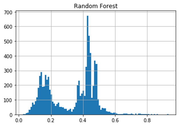
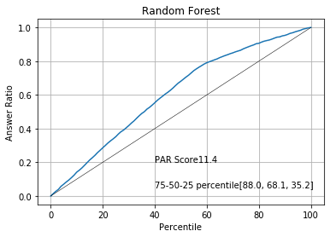
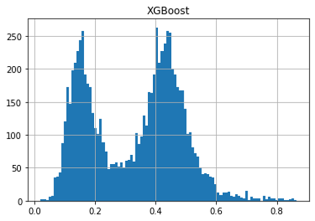
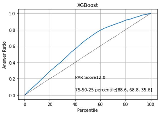


The PAR graphs show that we can expect the best result if we sort the data by the XGBoost model.
Conclusion
In this article we have documented the process of training several machine learning algorithms toward the end of calculating contactability scores. We used the scores to sort the phone number list and see which algorithm sorts the list the best toward the goal of minimizing the effort to contact a given set of numbers while getting the best results as quickly as possible.
Although PacificEast uses a hybrid of multiple approaches to build its CS model and therefore doesn t adhere to any single model documented, the end goal is the same in that we re producing a model that, if used to prioritize calling some numbers over others, increases contact rates while minimizing resources needed to make those calls and additionally reduced the number of calls people receive.
As a matter of implementation, our customers send us files containing the phone numbers they wish to call and we run them through our CS model which produces a score. When the scored file is returned to our customers, the sort the numbers by score (highest to lowest) and make calls in that order.
Our customers continue to successfully use our Contactability Score model to both minimize the number of number of calls made while maximizing contact rates.